Photometry Scaffolding

By Dr. Luisa Rebull, version 1, 19 Dec 2019, for Olivia and Tom

Attempting to work through scaffolding (after some preliminaries), going from single, isolated, point source with aperture fitting through clump of sources with PSF fitting.

Overview/Introduction

Many of the hiccups you are having may be coming from the fact that, by eye, you can see the sources *there* so what is the issue, but the gap in understanding has to do with explaining that to the computer in terms it can understand and mathematically reproduce identically each time.

Some web research (and consultations with other NITARP alumni) suggests that photometry resources on the web fall into two categories (1) overly simplified for basic concepts, or (2) throw you to the wolves in the context of masters’ or PhD work; figure it out on your own, buddy. So you’ve fallen in this legitimately present gap (crevasse?). I am not saying this is worth sharing with anyone else, or even maybe that helpful here, but here’s a go at filling that gap.

Key concept #1 – for a given image at a given time from a given telescope, at a given location on the chip, the PSF is the same for all sources, of all brightnesses, in the image. The telescope responds the same way to a point source of light regardless if it is bright or faint. For faint sources, you see just the peak of the function; for bright sources, you see lots more details, but it is the same shape as for faint sources.

• Ground-based, non-AO data are probably the same over the chip for a given exposure; if you’re lucky, it’s the same shape over the whole night, but if the weather changes, it’s not. Forget it being the same over a whole run.
• Ground-based, AO data are ~idealized but only over a tiny area on the chip. (one source at a time)
• Space-based data tend to be very, very stable, unless (and sometimes even though) the satellite heats/cools each orbit (e.g., HST). Usually diffraction-limited (Airy functions apparent).
• X-ray data tend to have a spatially-dependent PSF, e.g., the point sources on the edges are more elongated, and the point sources in the middle are more circular.

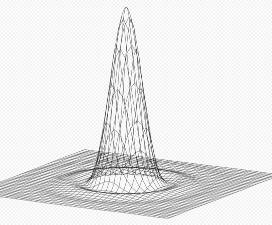
theoretical Airy function from Wikipedia.

PSFs – all of them – start as Airy functions, because physics. Atmosphere may smear them out. Pixels may be so big as to only “see” the highest part of it. Lots of additional effects may matter. Ex: Struts holding the secondary may cause additional diffraction.

Key concept #2 – There are a LOT of decisions to make. Every astronomer makes different decisions based on their experience, and every data set requires different decisions (e.g., space-based and ground-based data aren’t the same!). But give the same data to two different astronomers and they will get the same number, to within errors. If your two approaches (aperture and PSF) are not yielding the same number for the same source, somewhere your decisions are wrong. If your single approach is not yielding the same number for the same source (within errors) as someone else gets, someone’s decisions somewhere are wrong. But to assert that yours is right in that situation, you have to have a deep understanding of each of your decisions and know for a fact that they are right (and not just “good enough”). Ideally that someone else has written down somewhere exactly what they did so that you can pinpoint where your approaches differed, and why you think they did it wrong. (This is why I used the phrase “mathematically reproduce identically each time” above – it needs to be reproducible.) Two different measurements in the same band of the same target at different times may be legitimately different, because the object has changed. But start from the same data, and you better get the same number (within errors). The “within errors” is also important – if you make a decision early on, say not to center your source, then finer details of PSF structure doesn’t matter, because the errors are dominated by this centering issue. But understanding what the errors really are can save you grief agonizing over small details that don’t matter to within your errors. For our original project, we didn’t need photometry to 0.1% or 1% or even 10%. We were using the fluxes on a log-log SED and the magnitudes (also effectively log) in CMDs. 20% photometry (or even worse) is just fine for that. So the aperture photometry was totally good enough for what we were doing… except possibly for a few of the most crowded sources at the longer bands.

Key concept #3 – I’m not even going to approach flux calibration here. We’ll just assume our idealized cases are already flux-calibrated. For that matter, I’m going to ignore making mosaics too. This might matter (have mattered) for you because of whatever ImageJ did to your images; flux conservation is super important, but hopefully didn’t affect anything but edge pixels for you. Oh, and I’m assuming all basic processing has happened – flatfielding, etc., and that cosmic rays have been removed. (And assuming scattered light doesn’t matter.)

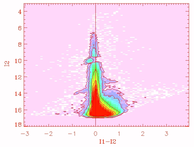
Key concept #4 – You should remember this from working with me – just because the computer says it, does not mean it is right. Do lots of checks at each possible step. Is what you’re doing making sense? Is it giving you weird results? Even if – especially if – you get to the end of what seems to be good decisions and you make a plot like this, you know immediately you have done something wrong. I don’t think I have EVER reduced data just once. Get used to the idea that you may be doing photometry on the same sources in the same image an uncountable number of times before you get it right.

(Look near I2~10 .. why have all of these source suddenly shifted left? Something is wrong.)

But once you get it right, more data from the same band and telescope will fly through. The second band from the same telescope/instrument will be easier than the first. Another instrument from the same telescope will be harder. Trying a new telescope? Go back to the start, do not pass Go, do not collect $200. But you’ll have a better sense of which parameters matter the most. Probably.

Single, isolated, ideal point source, aperture.

There is only one source. There is little or no background contribution. What are the decisions to make?

• a. Where is the source?
  • i. You tell it, this source is exactly here.
  • ii. You tell it, this source is here plus or minus a pixel; it finds the center.
  • iii. You let it find the sources and then center them.
  • iv. APT: you can click on it for an initial guess. You let the computer know that that is just a starting guess, and it still has to decide where the actual location is, to a fraction of a pixel.
  • v. If you let it find the source, in this idealized case, it will look for the brightest pixel (largest value) in the array.
  • vi. If you center your aperture a px off of the true center, will it matter? It might, depending on the size of the px and the PSF.
• b. How big should the aperture be to get “all the flux”?
  • i. Do you want a circular aperture, or a square? If the former, calculate flux over fractional px. How are you going to do that interpolation? If the latter, how does that compare to the actual PSF?
  • ii. For bright sources, you may need to go out a long way.
  • iii. For faint sources, going out far doesn’t make any sense, so you need smaller apertures.
  • iv. What happens if you don’t capture all the flux? Aperture corrections. How will you derive such a correction? (How did the Spitzer and Herschel staff do it?)
• c. Where should the annulus be (and how wide should it be) to get a good estimate of the background?
  • i. Circle? Or square? Recall fractional pixels above.
  • ii. How many pixels do you need to get a “good enough” estimate?
  • iii. How will you estimate the background? Mean? Median? Mode? A constant you determine via some other method? Something else?
  • iv. You estimated background per px over a number of px. Scale that to work for the px enclosed by your aperture (including fractional px).
• d. At the location of the source, drop the aperture, count up the flux, subtract off the scaled background estimate. Propagate errors to estimate uncertainties. Poisson statistics for the original electrons detected can propagate through the calibration process, so you should get an image full of errors along with fluxes. Then propagate that through the rest of the calculations.

Single, isolated, ideal point source, PSF.

As above: find the source, center the source. Then need new information about the PSF…

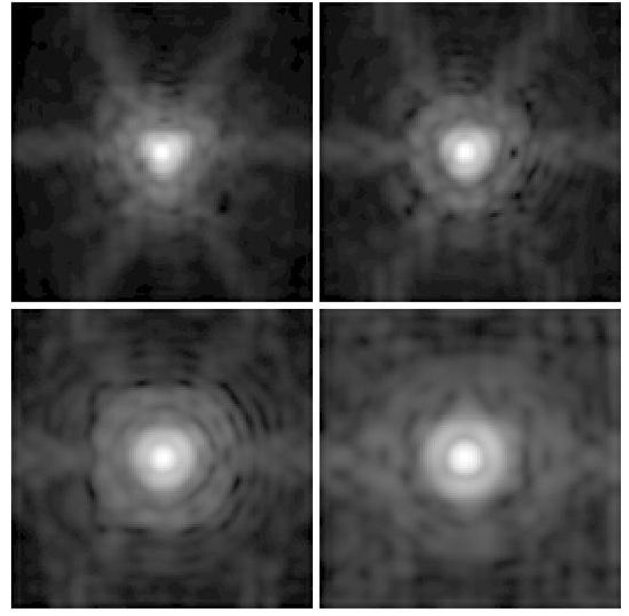
If you have ground-based, non-AO optical data, it may be Gaussian-ish. If you have anything else, it’s likely very complicated. Something has to hold the secondary in place, and light is a wave, so diffraction. Space-based data are often less variable than ground-based, but not necessarily. Rather than trying to guess the mathematical form of the theoretical PSF, use actual data to define your PSF. If you have ground-based data, this will be a function of time. If you have space-based data, it may be a function of time, or it may not be. You need a collection of quite a few bright, isolated stars to use to define your PSF. In-orbit checkout docs for IRAC suggest 300 observations went into their PSF (PRF) determination – go find Hoffman 2005 for gory detail, but results are copied here below.

Note too that for extremely precise IRAC photometry (exoplanets!) you need to know exactly which pixel your object fell on AND exactly where WITHIN THE PIXEL it fell. That whole discussion is super gory but look here if you want the full mess: https://irachpp.spitzer.caltech.edu/ Spitzer is a super-stable space-based magical machine. It was not ever designed for photometry even close to this precise. But it works.

Cryo IRAC PRFs. Note Airy ring most prominent in IRAC-4 (lower right) because wavelength the longest (and the telescope is the same over all four bands).

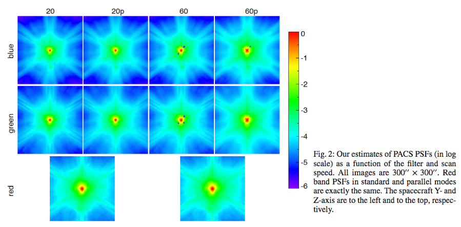
You may recall that PACS and SPIRE have PSFs that change slightly depending on scan speeds and direction. They need many examples of bright, isolated sources to sort that out. Bocchio et al. used asteroids.

PACS PSFs from Bocchio, Bianchi, & Abergel 2016. “20” and “60” are scan speeds in arcsec per sec. “P” means parallel (as opposed to scan) mode. RGB=160, 100, 70 um.

IRAS 12 um PSF.

IRAS scanned the whole sky but in the same direction every time. So, this is IRAS’s response to a point source (not an oblong source!) at 12 um. It’s a strong function of scan direction (it’s narrower in the scan direction).

Certainly when you go through this much work to get a PSF, you may wish to oversample your PSF so that you know in detail what the shape is. (e.g., use your 100s of sources to figure out the PSF shape at finer scale than the instrument’s native pixels).

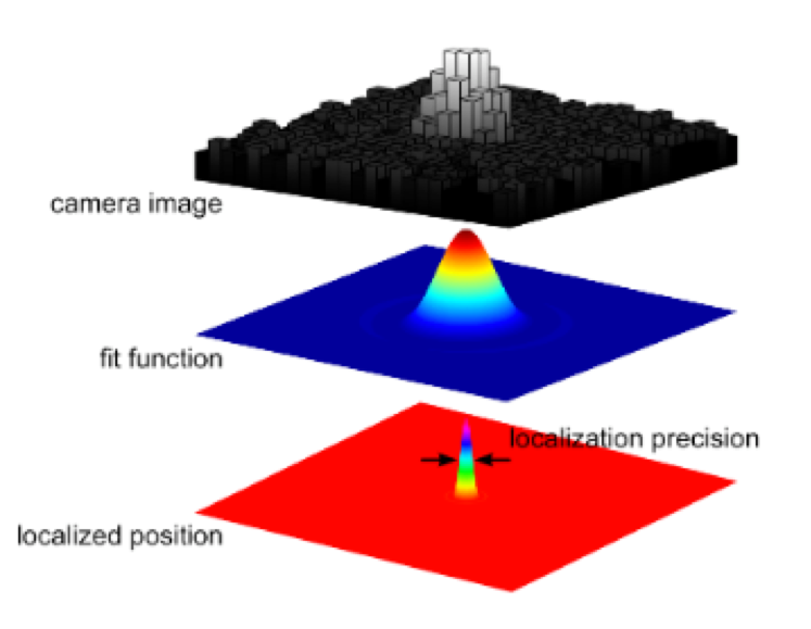
Now, you have a well-defined PSF and our idealized data for this example. Scale the PSF to match the data. How are you going to align them? Center location may not (will probably not) be an integer px. Your PSF is probably defined on integer px. How are you going to interpolate that to match scale, location of real data? (This is why you might want an oversampled PSF.) Once you do that, how are you going to match the data? You could just scale the PSF to the data at the peak value of the source. But then that only uses information from one px, and all of the PSFs I’ve shown you here cover >>1 px, and we should take advantage of that. After you’ve aligned the centers and interpolated the PSF to match the data at that location, then you need to scale it so that it fits “all the px.” How many are “all”? Down to what brightness level? Manually define some cutoff above which constitutes “source”? For this idealized example without (much) noise in the background, this seems easy. For all values above that, compare observed values to PSF values at each px, and minimize differences. For that fit, then can calculate observed brightness for that object.

Don't forget to calculate uncertainties on fit and total flux results. If you have a poorly-defined PSF (e.g., defined based on ~10 sources that may or may not be bright enough and may or may not be isolated and may or may not have ISM contributions), you are going to make life hard for yourself, and have larger errors than you would with a better-defined PSF.

How it works for many point sources, each of which are isolated, but with a variety of brightnesses, Aperture.

What are you going to do for all the sources in the image that are at a range of brightnesses?

Need to make a choice of the best aperture on average for most of the stars. Some will be too faint, some will be too bright, but most will be “good enough.” I had a hard time with this concept when I was learning, and tried to use variable apertures over my FOV. Just don’t do this. Pick something that is ‘typical’, use it for all the sources in the frame, and move on with your life. If you really need milli-magnitude precision, you’re probably not working on “all the sources” so go ahead and knock yourself out on your few sources and customize each measurement.

Don’t forget to make a good guess at errors.

How it works for many point sources, each of which are isolated, but with a variety of brightnesses, PSF.

You already know (key concept above) that all the PSFs are the same shape. Once you figure out how to do it for one, do it again for each source.

But, this starts to matter much more – how many px out of each source are you fitting? Down to what brightness level? Define a cutoff with respect to the background scatter? Measure the background scatter, care about pixels with excursions significantly above that level. (Define “significantly” -- 3 sigma? 5 sigma? 1 sigma?) For all values above that, compare observed values to PSF values at each px, and minimize differences, for each source. Astronomers usually use “reduced chi squared” to estimate goodness of fit and/or find the best fit.

Don’t forget to make a good guess at errors. Reduced chi square will help with that.

How it works for a single point source with variable background, aperture

So we still have a single source, but now the background variations matter lots more.

Source detection isn’t an issue here, yet, because we still have only one point source centered in our image.

To first order, then, the main impact is that you want an aperture relatively tightly centered on your source, and an aperture snugly into (up against) that. You don’t want too big an aperture that is set too far away, because then you won’t be sampling the background that is likely superimposed on your source at its location in the image. (You don’t want the aperture and annulus to overlap, because then you’l be counting the same photons.) And if the background is variable over scales smaller than your aperture/annulus, then you need to worry about how, exactly, you are calculating the background – mean, median, mode? Something else?

How it works for a single point source with variable background, PSF fitting

You need to tell the computer more specifically where the brightness cutoff level is for the fit. If you have a relatively faint source on a relatively bright background, you don’t want the computer using ISM brightnesses incorporated in its reduced chi squared fit, e.g., trying to fit the PSF wings to the ISM. So you have to be more careful in telling the computer the threshold above which it should fit. And don’t forget errors.

How it works for a collection of isolated point sources with variable background, aperture

Ok, now it starts to get more thorny. Out of the list above for a single isolated source, combined with the multiple source case, here is what now matters more than it did before:

Finding your source. Now that you’ve got a lot more sources to work with, you are not going to want to click on each one, nor do you necessarily have a list of sources already that it needs to do photometry. (Sometimes, actually, it is the case that you have a list of sources, in which case this step doesn’t matter; see far below.)

To find the sources, you need to teach the computer how to find sources. Usually, this means looking at the “typical” variations in the background, and then use the computer to look for brightness excursions beyond that fluctuation. This matters a lot, and there should be a parameter in units of that scatter that you can set to determine how deep you want to attempt source detection.

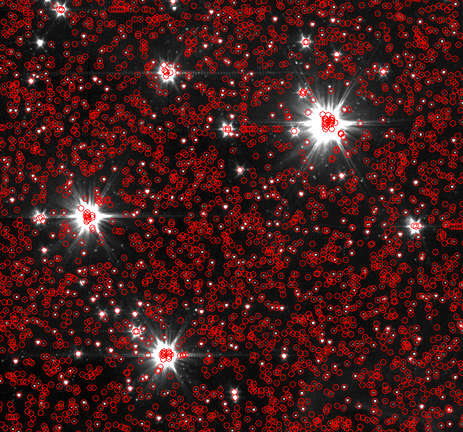
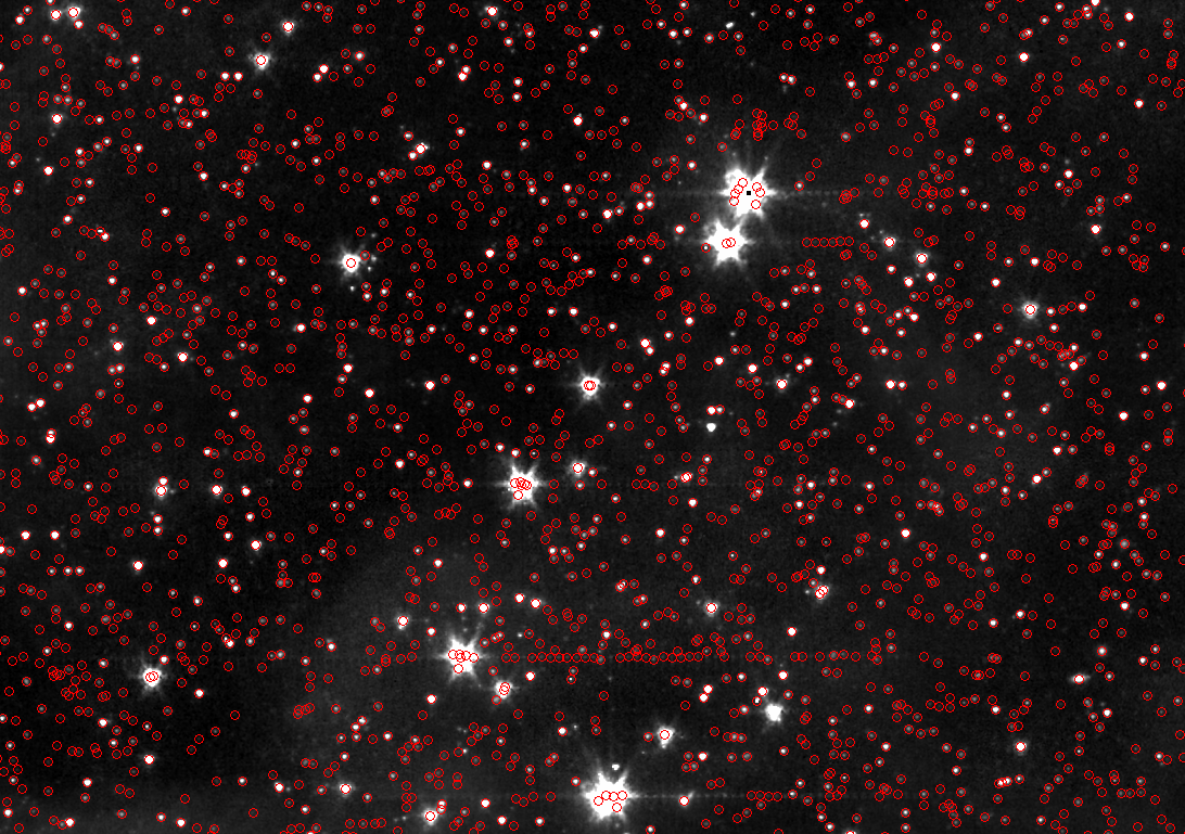Here is an example (MOPEX/APEX on an IRAC image) This source detection is actually doing pretty well, despite the variable background. Most of the sources you can see by eye are identified as such.

In most cases, it's doing pretty well - there is a real source visible within each red circle. BUT it clearly is having problems with the very bright and/or saturated sources, and it's detecting "sources" in the trail of image artifacts around the bright sources. I also see a resolved source in the lower right for which it has decided the central peak is a point source, and there are some legitimate point sources I can see by eye that the computer has not found.

There is definitely a point of diminishing returns -- you have to decide which objects you're interested in, how complete you want to be, and whether you can sustain “false” sources in this source list and/or missing sources in this source list. It could be that this is fine; if you’re going to match to sources from other wavelengths, false sources will fall away as having been detected in only one band, and sources in which you are interested that are missing from the source list can be manually added later. It could be, though, that you need to be more complete in the automatic extraction, in which case you need to get in and fiddle with the parameters. Interactive fiddling can make a big difference.

Here is another example (also MOPEX/APEX on an IRAC image). Why is it having trouble finding the fainter sources near the bright sources here? Can you figure out why it would struggle? (hint: background variations.)

Even though you are running source detection, it will still need you to tell it how much “slop” it has in centering each source, just like with the single sources above. This can be much smaller than when you are clicking on the source to give it an initial guess. But it still needs to be able to center each source properly.

You need to pick an aperture and annulus that works for all (most) of the sources in the image. And propagate errors through…

How it works for a collection of isolated point sources with variable background, PSF fitting

For this case, source detection is usually aided by the fact that it knows what the PSF looks like, so the chances of it, say, finding a “line” of false sources in a diffraction spike are greatly reduced, because it knows enough to figure out, hey, that’s a single pixel that’s bright in one dimension but not the other, so it’s probably not a point source. (For a bright ridge of nebulosity that is unresolved in one direction, you will likely get a line of "sources" along the ridge.) For an initial pass on the source detection, it is doing something very similar to what the aperture source detection is doing – it is looking for excursions above some threshold, and you have to pick the threshold appropriately for your data and your targets and your science goal.

MOPEX then takes the initial source detection and fitting, sorts the list by brightnesses, and then starts from the brightest source on the list. It takes the original image, fits the brightest source (as if it were an isolated source as above), and then subtracts it from the image. Repeat for the second source on the result of the first source’s subtraction. Repeat for each source. THEN go back through and do source detection on the residuals. Repeat.

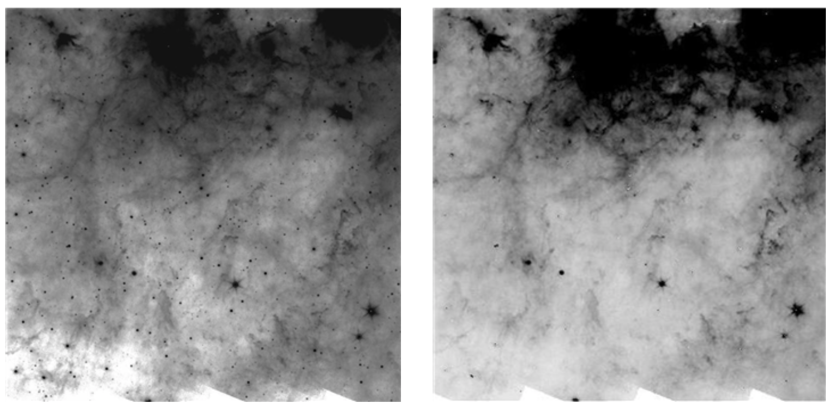MIPS example of PSF subtraction working.

Original image on left (lots of ISM because this is the galactic plane) Right is the same image having had all of the identified sources subtracted off. Note that it missed some of the brighter sources, but for the most part, the point sources are gone, and the residual, smooth ISM is left. That’s how you know that you’ve done a good job. If the second image had been filled with donuts, or the same number of point sources just fainter, or ISM with lots of neat (“precise” not “nifty”) holes punched in it (lawdy I have had many of those), then you know you did something wrong; go back and try different parameters or a better PSF or check the px scale of the PSF compared to your image… and propagate errors through …

How it works for a clump of sources very close to each other, aperture

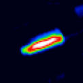
You should (hopefully) remember some of this from our work. In that context, we did not ask APT to determine where the sources were; we clicked on them in APT, or we (I) asked IDL to do photometry precisely at this RA and Dec. That knowledge came from us looking at other bands. We knew there were, say, 2 sources there, both kind of on top of each other given the PSF of the PACS70 data. This image here doesn’t even need information from other bands to tell us there are two sources –they’re a peanut shaped blob.

Because we were doing photometry for each source carefully, we could set the aperture for both of these centered tightly on the known position, put the annulus outside them both together, use that to get the same background for both of them, and use aperture corrections to bootstrap the tiny apertures to a full flux estimate. Doing this by hand is ok on a handful of sources, but it is rapidly tiresome for more than a few sources.

So, you want to go faster, more automatically (and thus more reproducibly). You can let it run source detection on its own over the image. But will it decide that this peanut above is one source or two? We know it’s two. The computer by itself might not figure that out, especially if the second star is much fainter than the first. The second star might look like an artifact and not show up as distinguishably a second source.. unless you are careful with the input parameters to the source detection.

You can also assemble a list of positions from other information, and give it a list of locations. (Be careful in that if you give it RA and Dec but the routine is expecting pixels, this is a problem. This is the case in my IDL code, so the first thing I do is translate RA and Dec to pixels in the image.)

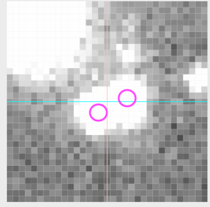
Because these sources are close together, you have to give it VERY LITTLE slosh for centering. The centering routines often assume there is only one source there. So if you give the computer working with the image above a centering tolerance of 3-4 px, both sources are likely to wander off their designated source position, and maybe even end up measuring exactly the same pixels for both sources… which clearly isn’t right.

So, what we did for the aperture photometry for our project is give it a list of positions that we know very well from other wavelengths, and did aperture photometry on those positions. (We used circular annuli close to the aperture, and used aperture corrections.)

How it works for a clump of sources very close to each other, PSF fitting

Same things apply wrt source detection here. It’s got a little better chance of working properly, because it knows what the PSF should look like, but you will probably have to help it by telling it that you know there are 4 sources at these locations, or whatever.

The reason (I suspect) that you are getting position wandering in what you are doing is that you are letting the computer determine where the sources are (both source detection and centering), and it is struggling with the precise location of the source given the big pixels (and sometimes undoubtedly neighbor proximity).

The way it should work for Ceph-C:

Isolated sources: aper and psf fitting should give the same result within errors, and both of those should match the published HPDP photometry for those cases where it is measured.

Close sources: give it a list of locations and find out what it comes back with – did it come back and tell you that it really thinks there is just one big source there and one faint one, even though you told it to start from a guess that there is 2? If it seems to have done it right, test it. Try image subtraction like MOPEX – is a smooth image what is left? Try adding points to SEDs – do they line up? Try making CMDs – are your nearby sources all in wrong places? If it doesn’t look good in any of these tests, go back and try different parameters.